On this page
Study guide
Try the problem before reviewing any worked steps or answers provided.
Trace breadth-first search, depth-first search, uniform-cost search and A* on the same graph. Then solve a minimax problem to see how search works when an opponent makes choices.
The graph and search rules
Start at S and find a path to goal G. Follow the arrows. The number on an edge is the cost of taking that step. Visit neighbours alphabetically and break equal priorities alphabetically.
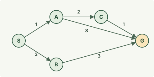
The frontier contains paths that have been found and are waiting to be explored. In the tables, the next node to remove is on the left. Stop when the goal is removed from the frontier. For recursive depth-first search, stop on the first visit to the goal.
Breadth-first search (BFS)
Problem. Find a path with the fewest edges. BFS uses a first-in, first-out queue. Mark each node when it joins the queue so it is queued once.
| Node removed | What happens | Queue after step |
|---|---|---|
| S | Discover A and B. | A, B |
| A | Discover C and G. | B, C, G |
| B | G is already queued. | C, G |
| C | G is already queued. | G |
| G | Goal reached. | Empty |
Result. The path is S → A → G. It has two edges and a cost of 1 + 8 = 9. BFS minimises the edge count. When costs differ, a longer path can be cheaper.
Depth-first search (DFS)
Problem. Find the first route reached by following each branch as far as possible. Use recursive DFS, marking a node when you enter it.
- At S, visit A first. The active path is S → A.
- At A, visit C before G. The active path is S → A → C.
- At C, visit G and stop. If C had been a dead end, backtrack to A and try its next neighbour.
Result. The path is S → A → C → G. It costs 1 + 2 + 1 = 4. DFS happens to find the cheapest path here because of the chosen neighbour order.
Uniform-cost search (UCS)
Problem. Find the cheapest route by choosing the lowest total cost so far, g(n). Keep the better path when the same node is reached with a lower cost.
| Node removed | Cost update | Frontier in g order |
|---|---|---|
| S (0) | Add A at 1 and B at 3. | A (1), B (3) |
| A (1) | Add C at 1 + 2 = 3 and G at 1 + 8 = 9. | B (3), C (3), G (9) |
| B (3) | Replace G’s cost of 9 with 3 + 3 = 6. | C (3), G (6) |
| C (3) | Replace G’s cost of 6 with 3 + 1 = 4. | G (4) |
| G (4) | Goal reached. | Empty |
Result. Follow G’s best predecessor back through C and A. The cheapest path is S → A → C → G, cost 4. Stopping when G first appears in the frontier would give cost 9.
A* search with a heuristic
Problem. Use the same graph and let h estimate the cost remaining to G. Use h(S) = 4, h(A) = 3, h(B) = 3, h(C) = 1 and h(G) = 0. At each step, choose the node with the lowest f(n) = g(n) + h(n).
| Node removed | New or improved scores | Frontier in f order |
|---|---|---|
| S (4) | A: 1 + 3 = 4. B: 3 + 3 = 6. | A (4), B (6) |
| A (4) | C: 3 + 1 = 4. G: 9 + 0 = 9. | C (4), B (6), G (9) |
| C (4) | G improves to 4 + 0 = 4. | G (4), B (6) |
| G (4) | Goal reached. | B (6) |
Result. A* also finds S → A → C → G, cost 4. It reaches the goal before expanding B. The heuristic here is consistent. For each edge, h at the source is at most the edge cost plus h at the destination. For example, h(A) = 3 and the edge A → C gives 2 + h(C) = 3.
Minimax with alpha–beta pruning
Problem. MAX can choose Left or Right. MIN then chooses between two outcomes. Left offers payoffs 3 and 5 to MAX. Right offers payoffs 2 and 9. Both players choose optimally.
- MIN chooses the lower payoff in each branch. Left is worth min(3, 5) = 3. Right is worth min(2, 9) = 2.
- MAX chooses max(3, 2) = 3, so Left is the best move.
- With alpha–beta pruning, evaluate Left first. MAX can already guarantee 3. In Right, the first leaf is 2, so MIN can hold MAX to at most 2 there. Skip the leaf with payoff 9.
For BFS and DFS, the frontier order determines which path is explored first. For UCS and A*, compare the scores before choosing the next node. For minimax, back up values from the leaves according to whose turn it is.